1. bidirectional transformer
2. pre-training objectives:
   1. masked language modeling完形填空 token-level
   2. next sentence prediction: s判断给出的两个Input sentence是否相邻 sentence-level

model architecture

BERT's model architecture is a multi-layer bidirectional Transformer encoder based on the original implementation described in Vaswani et al. (2017) and released in the tensor2tensor library. ${ }^{1}$

In this work, we denote the number of layers (i.e., Transformer blocks) as $L$, the hidden size as $H$, and the number of self-attention heads as $A .^{3}$ We primarily report results on two model sizes: BERT ${\text {BASE }}(\mathrm{L}=12, \mathrm{H}=768, \mathrm{~A}=12$, Total Parameters $=110 \mathrm{M})$ and $\mathbf{B E R T}{\mathbf{L A R G E}}(\mathrm{L}=24, \mathrm{H}=1024$, $\mathrm{A}=16$, Total Parameters $=340 \mathrm{M})$

input/output

input: a single sentence OR a pair of sentences

[cls] sentence1 [sep]sentence 2 [sep] ...

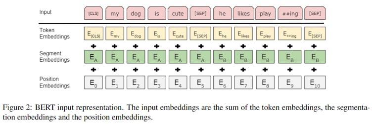
token embeddings, segment embeddings position embeddings都是通过学习得到的

pre-training

objective function

Task #1: Masked LM Intuitively, it is reasonable to believe that a deep bidirectional model is strictly more powerful than either a left-to-right model or the shallow concatenation of a left-toright and a right-to-left model. Unfortunately, standard conditional language models can only be trained left-to-right or right-to-left, since bidirectional conditioning would allow each word to indirectly "see itself", and the model could trivially predict the target word in a multi-layered context.

In order to train a deep bidirectional representation, we simply mask some percentage of the input tokens at random, and then predict those masked tokens. We refer to this procedure as a "masked LM" (MLM), although it is often referred to as a Cloze task in the literature (Taylor, 1953). In this case, the final hidden vectors corresponding to the mask tokens are fed into an output softmax over the vocabulary, as in a standard LM. In all of our experiments, we mask $15 \%$ of all WordPiece tokens in each sequence at random. In contrast to denoising auto-encoders (Vincent et al., 2008), we only predict the masked words rather than reconstructing the entire input.

Although this allows us to obtain a bidirectional pre-trained model, a downside is that we are creating a mismatch between pre-training and fine-tuning, since the [MASK] token does not appear during fine-tuning. To mitigate this, we do not always replace "masked" words with the actual [MASK ] token. The training data generator chooses $15 \%$ of the token positions at random for prediction. If the $i$-th token is chosen, we replace the $i$-th token with (1) the [MASK] token $80 \%$ of the time (2) a random token $10 \%$ of the time (3) the unchanged $i$-th token $10 \%$ of the time. Then, $T_{i}$ will be used to predict the original token with cross entropy loss. We compare variations of this procedure in Appendix C.2.

Task #2: Next Sentence Prediction (NSP) Many important downstream tasks such as Question Answering (QA) and Natural Language Inference $(\mathrm{NLI})$ are based on understanding the relationship between two sentences, which is not directly captured by language modeling. In order to train a model that understands sentence relationships, we pre-train for a binarized next sentence prediction task that can be trivially generated from any monolingual corpus. Specifically, when choosing the sentences A and B for each pretraining example, $50 \%$ of the time $\mathrm{B}$ is the actual next sentence that follows A (labeled as IsNext), and $50 \%$ of the time it is a random sentence from the corpus (labeled as NotNext). As we show in Figure 1, $C$ is used for next sentence prediction (NSP). ${ }^{5}$ Despite its simplicity, we demonstrate in Section $5.1$ that pre-training towards this task is very beneficial to both QA and NLI. ${ }^{6}$

dataset

The pre-training procedure largely follows the existing literature on language model pre-training. For the pre-training corpus we use the BooksCorpus (800M words) (Zhu et al., 2015) and English Wikipedia (2,500M words). For Wikipedia we extract only the text passages and ignore lists, tables, and headers. It is critical to use a document-level corpus rather than a shuffled sentence-level corpus such as the Billion Word Benchmark (Chelba et al., 2013) in order to extract long contiguous sequences.